Python

Drop Columns

函数 .drop()

# Drop some useless columns
to_drop = ['state','area_code','phone_number','churned']
churn_feat_space = churn_df.drop(to_drop, axis=1)

查看数据的unbalance

看true的比重

# check the propotion of y = 1
print(y.sum() / y.shape * 100)

Yes/No转换成True/False

# yes and no have to be converted to boolean values
yes_no_cols = ["intl_plan","voice_mail_plan"]
churn_feat_space[yes_no_cols] = churn_feat_space[yes_no_cols] == 'yes'

Gender转换成1/0

X_train['sex'] = (X_train.sex == 'M').astype(int)

Encoding Method

get_dummies()函数

在这里有各种encoding methods 最简单的其实就是.get_dummies()这个函数

pandas.get_dummies(data, prefix=None, prefix_sep='_', dummy_na=False, columns=None, sparse=False, drop_first=False)

drop_first: 其实是k-1个列就能表示k种情况，比如红蓝黄三种花，只需要2个column [1,0], [0,1], [0,0]

prefix : 转换后，列名的前缀

dummy_na : 增加一列表示空缺值，如果False就忽略空缺值

多个categorical feature在一列

如果一个column里一下放了好多个不同的categorical feature，想把它们提出来做encoding，这样可以提出来，画个图看一下每种里的数量

gen_split = TV['genres'].str.get_dummies(sep=',').sum()
gen_split.sort_values(ascending=False).plot.bar()

可以用两种方式做encode，然后再merge back

具体看这个链接

方式一

cleaned = df.set_index('video_id').genres.str.split(','), expand = True).stack()
cleaned = pd.get_dummies(cleaned, prefix = 'g').groupby(level=0).sum()

df = pd.merge(df, cleaned, on='video_id')
df.drop(['genres'], axis=1, inplace=True)

第二种方法更好读一点

方法二

genre = df['genres'].str.get_dummies(sep=',')
df = pd.merge(df.drop(columns=['genres'], genres, left_index=True, right_index=True, how='inner'))

如果有一些categorical feature实在太少，可以bin在一起，用| 或就行，或者是concat函数

d_genres['Misc_gen'] = d_genres['Anime']|d_genres['Reality']|d_genres['Lifestyle']|d_genres['Adult']|d_genres['LGBT']|d_genres['Holiday']
d_genres.drop(['Anime', 'Reality','Lifestyle', 'Adult','LGBT','Holiday'], inplace=True, axis=1)

newTV = pd.concat([TV_temp, d_import_id, d_mpaa, d_awards, d_genres, d_year], axis=1)

如果有很多个feature（比如国家，200个），那么可以用frequency作为encoder（简易版的target encoding）。

X_train['n_country_shared'] = X_train.country.map(X_train.country.value_counts(dropna=False))

年份的处理

如果是时间序列或者有年份的column，可以以10%~90%的percentile来bin年份为一个个bucket，最后把年份区间作为categorical feature做one-hot encoding。

用到的是cut这个函数，取前不取后

bin_year = [1916, 1974, 1991, 2001, 2006, 2008, 2010, 2012, 2013, 2014,2017]
year_range = ['1916-1974', '1974-1991', '1991-2001', '2001-2006','2006-2008','2008-2010','2010-2012','2012-2013',
              '2013-2014','2014-2017']
year_bin = pd.cut(TV['release_year'], bin_year, labels=year_range)
d_year = pd.get_dummies(year_bin).astype(np.int64)

Train_Test Split

注意如果data是unbalanced，可能在split的时候没有平均的分，所以在这个函数里有一个stratify选择true

另外如果面对“Train-Test Split“, "One Hot Encode", "SMOTE"等feature engineering的选项，第一个需要做的事一定是Train Test Split, 这样才不会让model偷看到Test的数据。

from sklearn import model_selection

# Reserve 20% for testing
X_train, X_test, y_train, y_test = model_selection.train_test_split(X, y, test_size=0.2)

print('training data has %d observation with %d features'% X_train.shape)
print('test data has %d observation with %d features'% X_test.shape)

Standardization/Normalization

注意如果要train-test split, 需要分别对这两个dataset做transformation 比如

fit transform 的mean和std拿到test上去用，但是不让train看到test里的值

standardization，目的是让数据在 （-1，1）（x-u）/sd, 对原始数据进行缩放处理，限制在一定的范围内。一般指正态化，即均值为0，方差为1。即使数据不符合正态分布，也可以采用这种方式方法，标准化后的数据有正有负。

normalization的目的是数据在（0，1）比如minmax scaling， (x-xmean)/(xmax-xmin)

这么做的目的是

1. 加速gradient descent

2. 把数据放在同一个scale里，让数据之间可以被比较，否则不同的feature会造成不同的影响

from sklearn.preprocessing import StandardScaler
scaler = StandardScaler()
X_train = scaler.fit_transform(X_train)
X_test = scaler.transform(X_test)

在实际做OA时一定要standardize，因为L1L2的系数，penalize的就不同 除了上面的standardscaler外，还有minmaxscalar、robustscalar

scaler = preprocessing.MinMaxScaler().fit(X_train[['n_dev_shared', 'n_ip_shared', 'n_country_shared']])
X_train[['n_dev_shared', 'n_ip_shared', 'n_country_shared']] = scaler.transform(X_train[['n_dev_shared', 'n_ip_shared', 'n_country_shared']])
X_test[['n_dev_shared', 'n_ip_shared', 'n_country_shared']] = scaler.transform(X_test[['n_dev_shared', 'n_ip_shared', 'n_country_shared']]) 

Classification Problem

Build Model and train

from sklearn.ensemble import RandomForestClassifier
from sklearn.neighbors import KNeighborsClassifier 
from sklearn.linear_model import LogisticRegression
from sklearn.svm import SVC 

# Logistic Regression
classifier_logistic = LogisticRegression()

# K Nearest Neighbors
classifier_KNN = KNeighborsClassifier()

# Random Forest
classifier_RF = RandomForestClassifier()

# SVM
classifier_SVC = SVC()

# Train the model
classifier_logistic.fit(X_train, y_train)

# Prediction of test data
classifier_logistic.predict(X_test)

# Accuracy of test data
classifier_logistic.score(X_test, y_test)

Cross Validation

# Use 5-fold Cross Validation to get the accuracy for different models
model_names = ['Logistic Regression','KNN','Random Forest', 'SVM']
model_list = [classifier_logistic, classifier_KNN, classifier_RF, classifier_SVC]
count = 0

for classifier in model_list:
    cv_score = model_selection.cross_val_score(classifier, X_train, y_train, cv=5)
    # cprint(cv_score)
    print('Model accuracy of %s is: %.3f'%(model_names[count],cv_score.mean()))
    count += 1

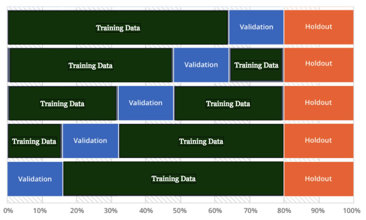
training的那一部分，继续分成五个小的dataset，每个小的dataset都做过training也都做过testing 把train_test_split理解为分出holdout data 见下图

注意上面的结构都是用的default hyper parameter

Hyperparameter Tuning

GridSearchCV

Grid-search： 比如，在random forest里，有两个hyper parameter，分别是depth和tree number，那么grid-search就是在排列组合

Grid-searchCV: 每个组合里再cross validation，比最后的mean score

from sklearn.model_selection import GridSearchCV

# helper function for printing out grid search results 
def print_grid_search_metrics(gs):
    print ("Best score: %0.3f" % gs.best_score_)
    print ("Best parameters set:")
    best_parameters = gs.best_params_
    for param_name in sorted(parameters.keys()):
        print("\t%s: %r" % (param_name, best_parameters[param_name]))

Logistic Regression Hyperparameter

C： inverse of lambda

# Possible hyperparamter options for Logistic Regression Regularization
# Penalty is choosed from L1 or L2
# C is the lambda value(weight) for L1 and L2
parameters = {
    'penalty':('l1', 'l2'), 
    'C':(1, 5, 10)
}
Grid_LR = GridSearchCV(LogisticRegression(),parameters, cv=5)
Grid_LR.fit(X_train, y_train)
best_LR_model = Grid_LR.best_estimator_

print_grid_search_metrics(Grid_LR)

KNN

# Possible hyperparamter options for KNN
# Choose k
parameters = {
    'n_neighbors':[3,5,7,10] 
    'max_depth':[3,5]
}
Grid_KNN = GridSearchCV(KNeighborsClassifier(),parameters, cv=5)
Grid_KNN.fit(X_train, y_train)

print_grid_search_metrics(Grid_KNN)

Random Forest

# Possible hyperparamter options for Random Forest
# Choose the number of trees
parameters = {
    'n_estimators' : [40,60,80]
}
Grid_RF = GridSearchCV(RandomForestClassifier(),parameters, cv=5)
Grid_RF.fit(X_train, y_train)
best_RF_model = Grid_RF.best_estimator_

print_grid_search_metrics(Grid_RF)

还可以写个wrapper，根据不同的scorer来筛选model

scorers = {
    'precision_score': make_scorer(precision_score),
    'recall_score': make_scorer(recall_score),
    'f1_score': make_scorer(f1_score, pos_label=1)
}

def grid_search_wrapper(model, parameters, refit_score='f1_score'):
    """
    fits a GridSearchCV classifier using refit_score for optimization(refit on the best model according to refit_score)
    prints classifier performance metrics
    """
#     skf = StratifiedKFold(n_splits=10)
#     grid_search = GridSearchCV(clf, param_grid, scoring=scorers, refit=refit_score,
#                            cv=skf, return_train_score=True, n_jobs=-1)
    grid_search = GridSearchCV(model, parameters, scoring=scorers, refit=refit_score,
                           cv=3, return_train_score=True, n_jobs=-1)
    grid_search.fit(X_train, y_train)

    # make the predictions
    y_pred = grid_search.predict(X_test)
    y_prob = grid_search.predict_proba(X_test)[:, 1]
    
    print('Best params for {}'.format(refit_score))
    print(grid_search.best_params_)

    # confusion matrix on the test data.
    print('\nConfusion matrix of Random Forest optimized for {} on the test data:'.format(refit_score))
    cm = confusion_matrix(y_test, y_pred)
    cmDF = pd.DataFrame(cm, columns=['pred_0', 'pred_1'], index=['true_0', 'true_1'])
    print(cmDF)
    
    print("\t%s: %r" % ("roc_auc_score is: ", roc_auc_score(y_test, y_prob)))
    print("\t%s: %r" % ("f1_score is: ", f1_score(y_test, y_pred)))#string to int

    print 'recall = ', float(cm[1,1]) / (cm[1,0] + cm[1,1])
    print 'precision = ', float(cm[1,1]) / (cm[1, 1] + cm[0,1])

    return grid_search

比如

Optimize F1 Score on LR

# C: inverse of regularization strength, smaller values specify stronger regularization
LRGrid = {"C" : np.logspace(-2,2,5), "penalty":["l1","l2"]}# l1 lasso l2 ridge
#param_grid = {'C': [0.01, 0.1, 1, 10, 100], 'penalty': ['l1', 'l2']}
logRegModel = LogisticRegression(random_state=0)

grid_search_LR_f1 = grid_search_wrapper(logRegModel, LRGrid, refit_score='f1_score')

Optimize F1 Score on RF

parameters = {        
'max_depth': [None, 5, 15],
'n_estimators' :  [10,150],
'class_weight' : [{0: 1, 1: w} for w in [0.2, 1, 100]]
}

clf = RandomForestClassifier(random_state=0)

grid_search_rf_f1 = grid_search_wrapper(clf, parameters, refit_score='f1_score')

best_rf_model_f1 = grid_search_rf_f1.best_estimator_

还可以把结果按照score sort了之后打印出来，precision, recall, f1等

results_f1 = pd.DataFrame(grid_search_rf_f1.cv_results_)
results_sortf1 = results_f1.sort_values(by='mean_test_f1_score', ascending=False)
results_sortf1[['mean_test_precision_score', 'mean_test_recall_score', 'mean_test_f1_score', 'mean_train_precision_score', 'mean_train_recall_score', 'mean_train_f1_score','param_max_depth', 'param_class_weight', 'param_n_estimators']].round(3).head()

按照feature importance排序一下

pd.DataFrame(best_rf_model_f1.feature_importances_, index = X_train.columns, columns=['importance']).sort_values('importance', ascending=False)

Model Evaluation

Confusion Matrix

from sklearn.metrics import confusion_matrix
from sklearn.metrics import classification_report
from sklearn.metrics import precision_score
from sklearn.metrics import recall_score

# calculate accuracy, precision and recall
def cal_evaluation(classifier, cm):
    tn = cm[0][0]
    fp = cm[0][1]
    fn = cm[1][0]
    tp = cm[1][1]
    accuracy  = (tp + tn) / (tp + fp + fn + tn + 0.0)
    precision = tp / (tp + fp + 0.0)
    recall = tp / (tp + fn + 0.0)
    print (classifier)
    print ("Accuracy is: %0.3f" % accuracy)
    print ("precision is: %0.3f" % precision)
    print ("recall is: %0.3f" % recall)

# print out confusion matrices
def draw_confusion_matrices(confusion_matricies):
    class_names = ['Not','Churn']
    for cm in confusion_matrices:
        classifier, cm = cm[0], cm[1]
        cal_evaluation(classifier, cm)
        fig = plt.figure()
        ax = fig.add_subplot(111)
        cax = ax.matshow(cm, interpolation='nearest',cmap=plt.get_cmap('Reds'))
        plt.title('Confusion matrix for %s' % classifier)
        fig.colorbar(cax)
        ax.set_xticklabels([''] + class_names)
        ax.set_yticklabels([''] + class_names)
        plt.xlabel('Predicted')
        plt.ylabel('True')
        plt.show()

%matplotlib inline

# Confusion matrix, accuracy, precison and recall for random forest and logistic regression
confusion_matrices = [
    ("Random Forest", confusion_matrix(y_test,best_RF_model.predict(X_test))),
    ("Logistic Regression", confusion_matrix(y_test,best_LR_model.predict(X_test))),
]

draw_confusion_matrices(confusion_matrices)

还采用的做法是可以把cm转换成df打印出来

cm = metrics.confusion_matrix(y_test, y_pred)
cmDF = pd.DataFrame(cm, columns=['pred_0', 'pred_1'], index=['true_0', 'true_1'])
print(cmDF)

ROC

from sklearn.metrics import roc_curve
from sklearn import metrics

# Use predict_proba to get the probability results of Random Forest
y_pred_rf = best_RF_model.predict_proba(X_test)[:, 1]
fpr_rf, tpr_rf, _ = roc_curve(y_test, y_pred_rf)

# ROC curve of Random Forest result
plt.figure(1)
plt.plot([0, 1], [0, 1], 'k--')
plt.plot(fpr_rf, tpr_rf, label='RF')
plt.xlabel('False positive rate')
plt.ylabel('True positive rate')
plt.title('ROC curve - RF model')
plt.legend(loc='best')
plt.show()

AUC

from sklearn import metrics

# AUC score
metrics.auc(fpr_rf,tpr_rf)

Feature Selection

L1

# add L1 regularization to logistic regression
# check the coef for feature selection
scaler = StandardScaler()
X_l1 = scaler.fit_transform(X)
LRmodel_l1 = LogisticRegression(penalty="l1", C = 0.1)
LRmodel_l1.fit(X_l1, y)
LRmodel_l1.coef_[0]
print ("Logistic Regression (L1) Coefficients")
for k,v in sorted(zip(map(lambda x: round(x, 4), LRmodel_l1.coef_[0]), \
                      churn_feat_space.columns), key=lambda k_v:(-abs(k_v[0]),k_v[1])):
    print (v + ": " + str(k))

L2

# add L2 regularization to logistic regression
# check the coef for feature selection
scaler = StandardScaler()
X_l2 = scaler.fit_transform(X)
LRmodel_l2 = LogisticRegression(penalty="l2", C = 5)
LRmodel_l2.fit(X_l2, y)
LRmodel_l2.coef_[0]
print ("Logistic Regression (L2) Coefficients")
for k,v in sorted(zip(map(lambda x: round(x, 4), LRmodel_l2.coef_[0]), \
                      churn_feat_space.columns), key=lambda k_v:(-abs(k_v[0]),k_v[1])):
    print (v + ": " + str(k))
  

就像feature selection的section所写，L1可以做feature selection，把correlation强的其中某项设置为0 而L2会把这两个做成近似的数值

Random Forest Feature Importance

# check feature importance of random forest for feature selection
forest = RandomForestClassifier()
forest.fit(X, y)

importances = forest.feature_importances_

# Print the feature ranking
print("Feature importance ranking by Random Forest Model:")
for k,v in sorted(zip(map(lambda x: round(x, 4), importances), churn_feat_space.columns), reverse=True):
    print (v + ": " + str(k))

注意这里的feature importance只是RF定义的importance，并不一定是物理意义上重要

Regression Problem

先用linear regression作为base model，在这里不一定非要用最简单的LR，可以直接上lasso和ridge，因为LR可以被认为是lambda=0时的lasso或者ridge。

Linear Regression

这里也涉及到调参，选择最优的lambda，可以画图来找 在下面的code中，x轴是lambda分之一的值，取值区间用了log space的150个点，因为这就能让前面的点相对密集，后面的点相对稀疏，更方便找到max（经验之谈）。

from sklearn.model_selection import train_test_split
from sklearn.linear_model import LinearRegression, Lasso, Ridge
from sklearn.metrics import mean_squared_error, r2_score
from math import sqrt

lr_train, lr_validate = train_test_split(model_train, test_size=0.15, random_state = 0)

lr_train_x = lr_train.drop(['video_id', 'cvt_per_day'], axis = 1)
lr_validate_x = lr_validate.drop(['video_id', 'cvt_per_day'], axis = 1)
lr_train_y = lr_train['cvt_per_day']
lr_validate_y = lr_validate['cvt_per_day']

alphas = np.logspace (-0.3, 2.5, num=150)
# alphas= [0.000000001]
scores = np.empty_like(alphas)
opt_a = float('-inf')
max_score = float('-inf')
for i, a in enumerate(alphas):
    lasso = Lasso()
    lasso.set_params(alpha = a)
    lasso.fit(lr_train_x, lr_train_y)
    scores[i] = lasso.score(lr_validate_x, lr_validate_y)
    if scores[i] > max_score:
        max_score = scores[i]
        opt_a = a
        lasso_save = lasso
plt.plot(alphas, scores, color='b', linestyle='dashed', marker='o',markerfacecolor='blue', markersize=6)
plt.xlabel('alpha')
plt.ylabel('score')
plt.grid(True)
plt.title('score vs. alpha')
plt.show()
print ('The optimaized alpha and score of Lasso linear is: ', opt_a, max_score)

然后train

# combine the validate data and training data, use the optimal alpha, re-train the model
lasso_f = Lasso()
lasso_f.set_params(alpha = opt_a)
lasso_f.fit(model_train_x, model_train_y)

# lasso_f is the Lasso model (linear feature), to be tested with final test data.

带Polynomial feature的LR

from sklearn.preprocessing import PolynomialFeatures

poly = PolynomialFeatures(2)

lr_train, lr_validate = train_test_split(model_train, test_size=0.15, random_state = 0)

lr_train_x = lr_train.drop(['video_id', 'cvt_per_day'], axis = 1)
lr_validate_x = lr_validate.drop(['video_id', 'cvt_per_day'], axis = 1)

lr_train_xp = poly.fit_transform(lr_train_x)
lr_validate_xp = poly.fit_transform(lr_validate_x)
lr_train_y = lr_train['cvt_per_day']
lr_validate_y = lr_validate['cvt_per_day']

# lr_train_xp = pd.DataFrame(data=lr_train_xp, index=data[:], columns=data[0,1:]) 

alphas = np.logspace (-2.6, 2.5, num=80)
# alphas= [1]
scores = np.empty_like(alphas)
opt_a = float('-inf')
max_score = float('-inf')
for i, a in enumerate(alphas):
    lasso = Lasso()
    lasso.set_params(alpha = a)
    lasso.fit(lr_train_xp, lr_train_y)
    scores[i] = lasso.score(lr_validate_xp, lr_validate_y)
    if scores[i] > max_score:
        max_score = scores[i]
        opt_a = a
        lasso_save = lasso
        
plt.plot(alphas, scores, color='b', linestyle='dashed', marker='o',markerfacecolor='blue', markersize=6)
plt.xlabel('alpha')
plt.ylabel('score')
plt.grid(True)
plt.title('score vs. alpha')
plt.show()
print ('The optimaized alpha and score of Lasso polynomial is: ', opt_a, max_score)

# combine the validate data and training data, use the optimal alpha, re-train the model
lr_train_xp1 = poly.fit_transform(model_train_x)

lasso_fp = Lasso()
lasso_fp.set_params(alpha = opt_a)
lasso_fp.fit(lr_train_xp1, model_train_y)

# lasso_fp is the Lasso model (polynomial feature), to be tested with test data.

然后train

# combine the validate data and training data, use the optimal alpha, re-train the model
lr_train_xp1 = poly.fit_transform(model_train_x)

lasso_fp = Lasso()
lasso_fp.set_params(alpha = opt_a)
lasso_fp.fit(lr_train_xp1, model_train_y)

# lasso_fp is the Lasso model (polynomial feature), to be tested with test data.

ridge也是同理

Non-Linear Model: Random Forest

from sklearn.ensemble import RandomForestRegressor
from sklearn.cross_validation import cross_val_score
from sklearn.model_selection import cross_validate
# from sklearn.grid_search import GridSearchCV
from sklearn.model_selection import GridSearchCV

rf_train, rf_test = train_test_split(model_train, test_size=0.15, random_state = 0)

rf_train_x = rf_train.drop(['video_id', 'cvt_per_day'], axis = 1)
rf_test_x = rf_test.drop(['video_id', 'cvt_per_day'], axis = 1)
rf_train_y = rf_train['cvt_per_day']
rf_test_y = rf_test['cvt_per_day']

param_grid = {
                 'n_estimators': [54, 55, 56, 57, 58, 59, 60, 62],
                 'max_depth': [12, 13, 14, 15, 16, 17]
             }

rf = RandomForestRegressor(random_state=2, max_features = 'sqrt')
grid_rf = GridSearchCV(rf, param_grid, cv=5)
grid_rf.fit(rf_train_x, rf_train_y)

最后出来的这个grid_rf下有一个非常重要的best_params_，能输出最佳的hyper parameter数值

grid_rf.best_params_

另外，还有一个重要的结果是cv_results_下的内容，其中有一个'mean_test_score'记录了test scores，可以在图上画出来，找最高点

# plot the effect of different number of trees and maximum tree-depth druing cross validation 
scores = grid_rf.cv_results_['mean_test_score']

n_est = [54, 55, 56, 57, 58, 59, 60, 62]
m_depth=[12, 13, 14, 15, 16, 17]
scores = np.array(scores).reshape(len(m_depth), len(n_est))
fig = plt.figure()
ax = plt.subplot(111)
for ind, i in enumerate(m_depth):
    plt.plot(n_est, scores[ind], '-o', label='M Depth' + str(i),)
    
ax.legend(loc='center left', bbox_to_anchor=(1, 0.5))
plt.xlabel('N Trees')
plt.ylabel('Mean Scores')
plt.grid(True)
plt.show()
# savefig('rf_1')

接下来就能根据图像找到点、重新train

# add both training and validation data together as the new training data
rf = RandomForestRegressor(random_state=2, max_features = 'sqrt', max_depth= 14, n_estimators=55)
rf.fit(model_train_x, model_train_y)

Model Evaluation, score, mean squared error

Lasso, Linear

# Lasso_f test (with linear features)

lasso_f_score = lasso_f.score(model_test_x, model_test_y)
pred_y = lasso_f.predict(model_test_x)

# The mean squared error and root mean square error
MSE_lasso_f = mean_squared_error(model_test_y, pred_y)
RMSE_lasso_f = sqrt(mean_squared_error(model_test_y, pred_y))

print ('lasso_f score: ', lasso_f_score)
print ('Mean square error of lasso_f: ', MSE_lasso_f)
print ('Root mean squared error of lasso_f:', RMSE_lasso_f)
# print ('Coefficients of lasso_f: ', lasso_f.coef_)

Ridge, poly

# ridge_fp test (with polynomial features)
model_test_xp = poly.fit_transform(model_test_x)

ridge_fp_score = ridge_fp.score(model_test_xp, model_test_y)
MSE_ridge_fp = mean_squared_error(model_test_y, pred_y)
RMSE_ridge_fp = sqrt(mean_squared_error(model_test_y, pred_y))

pred_y = ridge_fp.predict(model_test_xp)
print ('ridge_fp score: ', ridge_f_score)
print ('Mean square error of ridge_fp: ', MSE_ridge_fp)
print ('Root mean squared error of ridge_fp:', RMSE_ridge_fp)
#print ('Coefficients of ridge_fp: ', ridge_fp.coef_)

可以把这些都画在图上，直观看到最高的 不过因为只有五个点而已，画图可能不好看，表格也许更直观

lst_score = [lasso_f_score, lasso_fp_score, ridge_f_score, ridge_fp_score, rf_score]
MSE_lst =  [MSE_lasso_f, MSE_lasso_fp, MSE_ridge_f, MSE_ridge_fp, MSE_rf]
RMSE_lst =  [RMSE_lasso_f, RMSE_lasso_fp, RMSE_ridge_f, RMSE_ridge_fp, RMSE_rf]
model_lst = ['Lasso_linear','Lasso poly', 'Ridge linear', 'Ridge poly', 'Random forest']

plt.figure(1)
plt.plot(model_lst, lst_score, 'ro')
plt.legend(loc = 9)
plt.legend(['r-squre / score'])
plt.xlabel('model names',fontsize =16)
plt.ylabel('score / r square', fontsize =16)
plt.grid(True)
plt.show()

plt.figure(2)
plt.plot(model_lst, MSE_lst, 'g^')
plt.legend(loc = 9)
plt.legend(['mean square error (MSE)'])
plt.xlabel('model names', fontsize =16)
plt.ylabel('mean square error', fontsize =16)
plt.grid(True)
plt.show()

plt.figure(3)
plt.plot(model_lst, RMSE_lst, 'bs')
plt.legend(loc = 9)
plt.legend(['root mean square error (RMSE)'])
plt.xlabel('model names', fontsize =16)
plt.ylabel('root mean square error', fontsize =16)
plt.grid(True)
plt.show()

Feature Importance with Random Forest

importances = rf.feature_importances_
std = np.std([tree.feature_importances_ for tree in rf.estimators_], axis=0)
indices = np.argsort(importances)[::-1]
feature_name = model_test_x.columns.get_values()

# Print the feature ranking
print("Feature importance ranking:")

for f in range(model_test_x.shape[1]):
    print("%d. feature %d %s (%f)" % (f + 1, indices[f],  feature_name[f], importances[indices[f]]))
    
plt.figure(1)
plt.bar(feature_name[:11], importances[indices[:11]])
plt.xticks(rotation=90)
plt.show()

也是一样可以画图看

在上面的code block里第三行的函数argsort，是numpy中的quicksort，可以沿着axis=0(列）或者axis=1（行）排序，输出是从小到大的索引 如果想要获得从大到小，可以np.argsort(-x)，或者[::-1]

第四行model_test_x.columns.get_values()可以方便地获取column的名字

Unsupervised Learning

K-means clustering

# k-means clustering
from sklearn.cluster import KMeans

# number of clusters
num_clusters = 5
km = KMeans(n_clusters=num_clusters)
km.fit(tfidf_matrix)
clusters = km.labels_.tolist()

# create DataFrame films from all of the input files.
films = { 'title': titles, 'rank': ranks, 'synopsis': synopses, 'cluster': clusters}
frame = pd.DataFrame(films, index = [clusters] , columns = ['rank', 'title', 'cluster'])

print ("Number of films included in each cluster:")
frame['cluster'].value_counts().to_frame()

print ("<Document clustering result by K-means>")

#km.cluster_centers_ denotes the importances of each items in centroid.
#We need to sort it in decreasing-order and get the top k items.
order_centroids = km.cluster_centers_.argsort()[:, ::-1] 

Cluster_keywords_summary = {}
for i in range(num_clusters):
    print ("Cluster " + str(i) + " words:", end='')
    Cluster_keywords_summary[i] = []
    for ind in order_centroids[i, :6]: #replace 6 with n words per cluster
        Cluster_keywords_summary[i].append(vocab_frame_dict[tf_selected_words[ind]])
        print (vocab_frame_dict[tf_selected_words[ind]] + ",", end='')
    print ()
    #Here ix means index, which is the clusterID of each item.
    #Without tolist, the values result from dataframe is <type 'numpy.ndarray'>
    cluster_movies = frame.ix[i]['title'].values.tolist()
    print ("Cluster " + str(i) + " titles (" + str(len(cluster_movies)) + " movies): ")
    print (", ".join(cluster_movies))
    print ()

plot the result

# use pca to reduce dimensions to 2d for visibility, just want to see if there 2d can give us some insights
# this is not an appropriate method, just a guess.
pca = decomposition.PCA(n_components=2)
tfidf_matrix_np=tfidf_matrix.toarray()
pca.fit(tfidf_matrix_np)
X = pca.transform(tfidf_matrix_np)

xs, ys = X[:, 0], X[:, 1]

#set up colors per clusters using a dict
cluster_colors = {0: '#1b9e77', 1: '#d95f02', 2: '#7570b3', 3: '#e7298a', 4: '#66a61e'}
#set up cluster names using a dict
cluster_names = {}
for i in range(num_clusters):
    cluster_names[i] = ", ".join(Cluster_keywords_summary[i])

# %matplotlib inline 

#create data frame with PCA cluster results
df = pd.DataFrame(dict(x=xs, y=ys, label=clusters, title=titles)) 
groups = df.groupby(clusters)

# set up plot
fig, ax = plt.subplots(figsize=(16, 9))
#Set color for each cluster/group
for name, group in groups:
    ax.plot(group.x, group.y, marker='o', linestyle='', ms=12, 
            label=cluster_names[name], color=cluster_colors[name], 
            mec='none')

ax.legend(numpoints=1,loc=4)  #show legend with only 1 point, position is right bottom.

plt.show() #show the plot